

Monocular depth estimation is a pc imaginative and prescient process the place an AI mannequin tries to foretell the depth info of a scene from a single picture. On this course of, the mannequin estimates the space of objects in a scene from one digicam viewpoint. Monocular depth estimation has many purposes and has been broadly utilized in autonomous driving, robotics, and extra. Depth estimation is taken into account one of many hardest pc imaginative and prescient duties, because it requires the mannequin to grasp complicated relationships between objects and their depth info. This implies many elements come into play when estimating the depth of a scene. Lighting circumstances, occlusion, and texture can drastically have an effect on the outcomes.
We’ll discover monocular depth estimation to grasp the way it works, the place it’s used, and implement it with Python tutorials. So, let’s get began.
About us: Viso Suite is end-to-end pc imaginative and prescient infrastructure for enterprises. Housed in a single platform, groups can handle a variety of duties from individuals counting to object detection and motion estimation. To see how Viso Suite can profit your group, e-book a demo with our workforce of consultants.
Understanding Monocular Depth Estimation
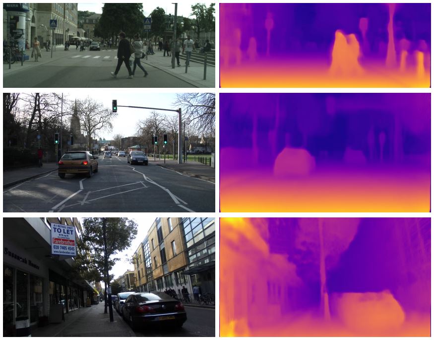
Depth estimation is a vital step in direction of understanding scene geometry from 2D photographs. The objective of monocular depth estimation is to foretell the depth worth of every pixel. That is referred to as inferring depth info, utilizing just one RGB enter picture. Depth estimation methods analyze visible particulars reminiscent of perspective, shading, and texture to estimate the relative distances of objects in an Picture. The output of a depth estimation mannequin is usually a depth map.
To coach AI fashions on depth-maps we are going to first need to generate depth-maps. Depth estimation is a process that helps machines see the world in 3D, identical to we do. This provides us an correct sense of distances and enhances our interactions with our environment. We use just a few frequent applied sciences to generate depth maps with cameras. For instance, Time-of-Flight and Mild Detection and Ranging (LiDAR), are standard depth-sensing applied sciences engineers use in fields like robotics, industrial automation, and autonomous automobiles. Subsequent, let’s clarify these necessary pc imaginative and prescient (CV) applied sciences.
How Does Depth Estimation Work?
Throughout the world of depth sensing applied sciences there isn’t any single answer to each software, in some instances, engineers might even use a mix of strategies to attain the specified outcomes. A robotic or an autonomous automobile can use cameras and sensors with embedded software program to sense depth info using standard strategies. These strategies normally include a sign that may be something from gentle or sound to particles. Then some algorithms are utilized to calculate the Time-of-flight and extract info from that.
A great instance is stereo depth estimation, in contrast to monocular depth estimation it really works by utilizing 2 cameras with sensors taking photographs in parallel. That is like human binocular imaginative and prescient as a result of engineers set two cameras just a few centimeters aside. The embedded software program detects the matching options within the photographs. Since every picture can have a distinct offset of the detected options, the software program makes use of the offset to calculate the depth of the purpose by way of a way referred to as triangulation.
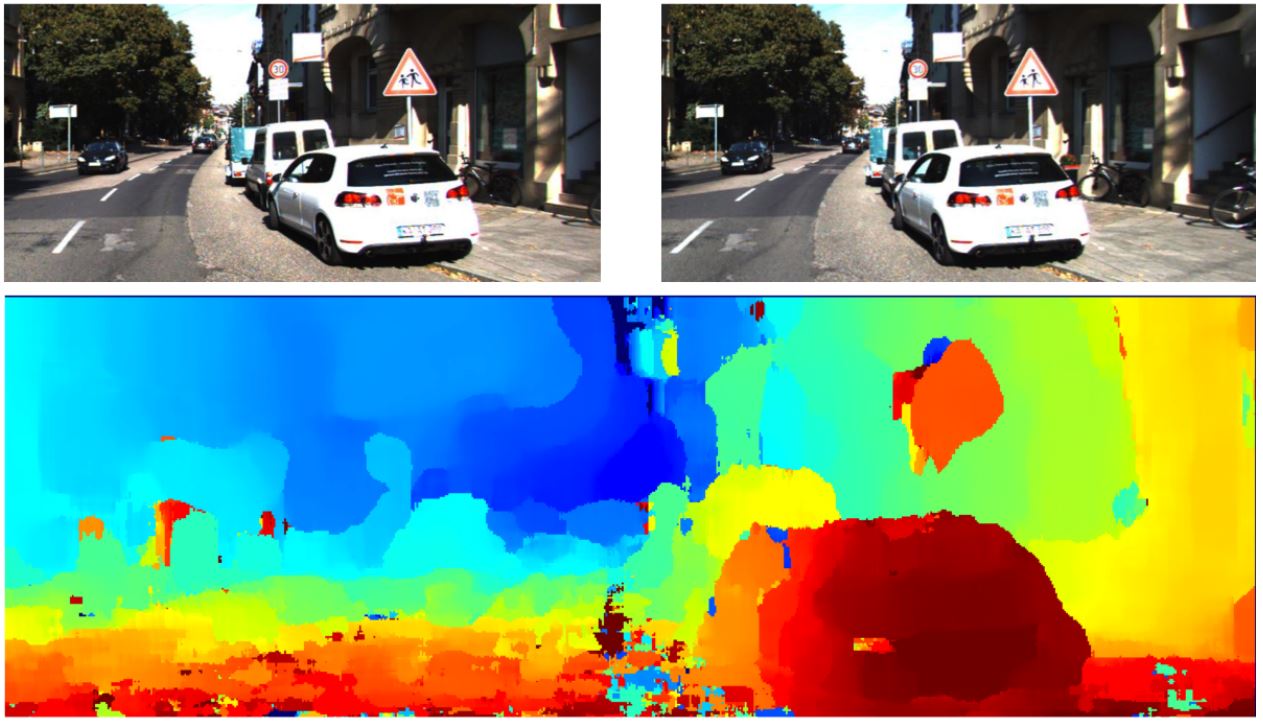
Most stereo-depth cameras use lively sensing and a patterned gentle projector, that casts a sample on surfaces, that helps determine flat or textureless objects. These cameras usually use near-infrared (NIR) sensors, enabling them to detect each the projected infrared sample and visual gentle. Different methods like LiDAR use gentle within the type of a laser that activates and off quickly to measure distances from which software program can calculate depth measurements. That is typically utilized in creating 3D maps of locations, it may be used to discover caves, historic websites, and any earth floor. However, monocular depth estimation depends on utilizing one picture to foretell the depth map, utilizing AI methods for correct predictions. Let’s have a look at the totally different AI methods utilized in monocular depth estimation.
AI Strategies In Monocular Depth Estimation
Whereas stereo depth estimation methods are helpful for some eventualities, developments in synthetic intelligence have opened the door for brand spanking new use instances of depth estimation, reminiscent of monocular depth estimation. With the ability of machine studying engineers can practice and infer machine studying fashions to foretell depth maps from a single picture. This in flip led to developments in fields like autonomous driving, and augmented actuality. The principle benefit is that specialised gear shouldn’t be wanted to sense the depth of knowledge. On this part, we are going to discover the AI methods used for monocular depth estimation.
Supervised Studying for Monocular Depth Estimation
Synthetic neural networks (ANNs) since their invention have been instrumental in fixing issues like monocular depth estimation. There are a number of methods a neural community may be educated, and a kind of is supervised studying. In supervised studying, the mannequin is educated on knowledge with labels, the place a neural community can study relationships between the photographs and their depth maps, and make predictions based mostly on the discovered relationships. Researchers broadly use convolutional neural networks (CNNs). CNNs can study an implicit relation between colour pixels and depth. Mixed with post-processing and deep-learning approaches CNNs are actually probably the most broadly used spine for depth estimation fashions.
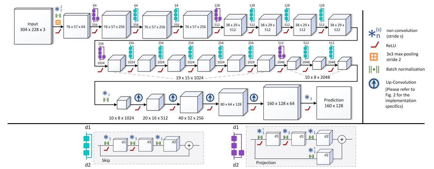
Since constructing and coaching these CNNs is a tough process, researchers normally use a pre-trained mannequin and apply the necessary idea of switch studying. Switch studying is utilized to a mannequin that has been educated on a basic dataset to make it work for a extra particular use case. Some standard U-net-based architectures that researchers use as backbones for fine-tuned monocular depth estimation fashions are the next.
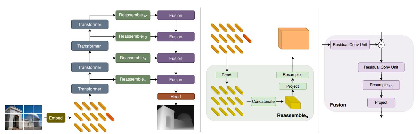
Nevertheless, extra fashionable structure may be Imaginative and prescient Transformers (ViT), these transformative fashions have been launched as alternate options to CNNs in pc imaginative and prescient purposes. ViTs use a self-attention block within the structure permitting it to have the next capability and lead to superior efficiency. These fashions principally depend on an encoder-decoder structure that may be made into totally different variations for various use instances. In comparison with CNN-based architectures, ViT-based ones have greater than a 28% efficiency improve in depth estimation.
Whereas these strategies work nice with supervised studying, they rely closely on massive labeled datasets that are costly, time-consuming, and may have biases. Subsequent, let’s discover different coaching strategies.
Unsupervised and Self-Supervised Studying for Monocular Depth Estimation
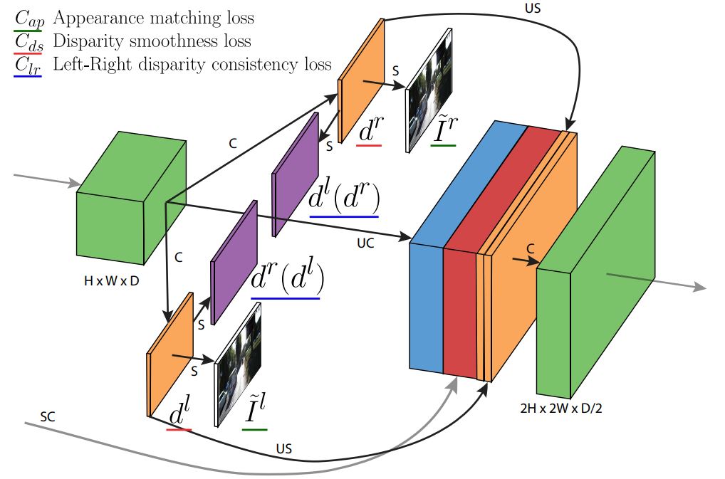
Most monocular depth estimation approaches deal with depth prediction as a supervised regression downside and consequently, require huge portions of ground-truth depth knowledge for coaching. Nevertheless, different unsupervised and self-supervised approaches obtain nice ends in depth prediction with easier-to-obtain binocular stereo footage. Researchers can leverage stereo-image pairs in the course of the mannequin’s coaching to permit neural networks to study implicit relations between the pairs.
The core thought is to coach the community to reconstruct one picture of the stereo pair from the opposite. By studying to do that, the community implicitly learns concerning the depth of the scene. Mixed with different approaches like left-right consistency unsupervised approaches can lead to state-of-the-art efficiency. Left-right consistency permits the community to foretell disparity maps for each the left and proper photographs, and the coaching loss encourages these disparity maps to be in line with one another.
Self-supervised studying is one other method researchers have taken for depth estimation. One of many standard research makes use of a video sequence to coach the neural community. The neural community learns the distinction between body A and body B utilizing pose estimation. The community tries to reconstruct body B from body A, evaluate the reconstruction, and decrease the error. Moreover, the researchers of this research used just a few methods to enhance the efficiency.
These methods embrace auto-masking the place objects which might be stationary in each body are masked to not confuse the mannequin, and full-resolution multi-scale to enhance high quality and accuracy. That being stated, depth-estimation approaches are continuously evolving, and researchers are discovering new methods to make correct depth maps from single photographs. So, subsequent, let’s get right into a step-by-step tutorial to construct a depth-estimation mannequin.
Step-by-Step Tutorial: Utilizing a Depth Estimation Mannequin
Now that we now have explored the theoretical ideas of monocular depth estimation, let’s roll up our sleeves for a sensible implementation with Python. On this tutorial, we are going to undergo the method of constructing and utilizing a depth estimation mannequin. We will likely be using the Keras framework with Tensorflow, and constructing upon the supplied instance by Keras. Nevertheless, some prior data of Python and machine studying ideas will likely be helpful for this part. On this instance, we’ll adapt and enhance upon the code from the Keras tutorial on monocular depth estimation and we’ll construction it as follows.
- Setup and Knowledge Preparation
- Constructing the Knowledge Pipeline
- Constructing the Mannequin and Defining the Loss
- Mannequin Coaching and Inference
So, let’s begin with the setup and knowledge preparation for this tutorial.
Setup and Knowledge Preparation
For this tutorial, we are going to use Kaggle as our surroundings and the Dense Indoor and Out of doors Depth (DIODE) Dataset to coach our mannequin. So, let’s begin by making ready our surroundings and importing the wanted libraries. I created a brand new Kaggle pocket book and enabled GPU acceleration.
import os
os.environ["KERAS_BACKEND"] = "tensorflow"
import sys
import tensorflow as tf
import keras
from keras import layers
from keras import ops
import pandas as pd
import numpy as np
import cv2
import matplotlib.pyplot as plt
keras.utils.set_random_seed(123)
These imports give us all of the libraries we’d like for the monocular depth estimation mannequin. We’re utilizing the OS, SYS, OpenCV (CV2) Tensorflow, Keras, Numpy, Pandas, and Matplot. Keras and TensorFlow are going to be the backend, OS and SYS will assist us with knowledge loading, CV2 will assist us course of the photographs, and Numpy and Pandas to facilitate between the loading and processing.
Subsequent, let’s obtain the info, as talked about beforehand we are going to use the DIODE dataset, nonetheless, we are going to solely use the validation dataset as a result of the complete dataset is over 80GB which is just too massive for our objective. The validation knowledge is 2.6GBs which is simpler to deal with and higher for our objective so we are going to use that.
annotation_folder = "/kaggle/working/dataset/"
if not os.path.exists(os.path.abspath(".") + annotation_folder):
    annotation_zip = keras.utils.get_file(
        "val.tar.gz",
        cache_subdir=os.path.abspath(annotation_folder),  # Extract to /kaggle/working/dataset/
        origin="http://diode-dataset.s3.amazonaws.com/val.tar.gz",
        extract=True,
    )
This code downloads the validation set of the DIODE dataset to the Kaggle/working folder, and it’ll extract it in a folder referred to as dataset in there. So, now we now have the dataset put in in our Kaggle workspace. Subsequent, let’s put together this knowledge and course of it to turn into appropriate to be used in coaching our mannequin.
df_list = [] # To Retailer Each Indoor and Out of doors
for scene_type in ["indoors", "outdoor"]:
    path = os.path.be a part of("/kaggle/working/dataset/val", scene_type)
    filelist = []
    for root, dirs, information in os.stroll(path):
        for file in information:
            filelist.append(os.path.be a part of(root, file))
    filelist.kind()
    knowledge = {
        "picture": [x for x in filelist if x.endswith(".png")],
        "depth": [x for x in filelist if x.endswith("_depth.npy")],
        "masks": [x for x in filelist if x.endswith("_depth_mask.npy")],
    }
    df = pd.DataFrame(knowledge)
    df = df.pattern(frac=1, random_state=42)
    df_list.append(df)  # Append the dataframe to the listing
# Concatenate the dataframes
df = pd.concat(df_list, ignore_index=True)
#Verify if Paths are appropriate
print(df.iloc[0]['image'])
print(df.iloc[0]['depth'])
print(df.iloc[0]['mask'])
Don’t be intimidated by the code, what this principally does is it goes by way of the information we downloaded, and appends the file names right into a Pandas knowledge body. Since we will likely be utilizing each indoor and out of doors photographs from the dataset we use 3 For loops, that first undergo the indoors folder, we put the “.png” picture information in a column, the depth values in a column, and the masks in one other.
Constructing The Knowledge Pipeline
For monocular depth estimation, we use the depth values and the masks to generate a depth map that we are going to use to coach the mannequin alongside the unique photographs. We’ll construct a pipeline perform that basically does the next.
- Learn a Pandas knowledge body with paths for the RGB picture, the depth, and the depth masks information.
- Load and resize the RGB photographs.
- Reads the depth and depth masks information, processes them to generate the depth map picture, and resizes it.
- Return the RGB photographs and the depth map photographs for every batch.
Usually in machine studying, knowledge pipelines are constructed as courses, this makes it simpler to make use of the pipeline as many instances as wanted. On this tutorial, we are going to construct it as a perform that makes use of some standard knowledge processing strategies that may assist us practice our mannequin effectively.
def load_and_preprocess_data(df_row, img_size=(256, 256)):
    """
    Masses and preprocesses picture and depth map from a DataFrame row
    """
    img_path = df_row['image']
    depth_path = df_row['depth']
    mask_path = df_row['mask']

    img = cv2.imread(img_path)
    img = cv2.cvtColor(img, cv2.COLOR_BGR2RGB)
    img = cv2.resize(img, img_size)
    img = tf.picture.convert_image_dtype(img, tf.float32) # Use tf.picture.convert_image_dtype
    depth_map = np.load(depth_path).squeeze()
    masks = np.load(mask_path)
    masks = masks > 0
    max_depth = min(300, np.percentile(depth_map, 99))
    depth_map = np.clip(depth_map, 0.1, max_depth)
    depth_map = np.log(depth_map, the place=masks)
    print("Min/Max depth earlier than preprocessing:", np.min(depth_map), np.max(depth_map))
    depth_map = np.ma.masked_where(~masks, depth_map)
    depth_map = np.clip(depth_map, 0.1, np.log(max_depth))# Clip after masking
    depth_map = cv2.resize(depth_map, img_size)
    depth_map = np.expand_dims(depth_map, axis=-1)
    depth_map = tf.picture.convert_image_dtype(depth_map, tf.float32)
    print("Min/Max depth after preprocessing:", np.min(depth_map), np.max(depth_map))# Use tf.picture.convert_image_dtype
    return img, depth_map
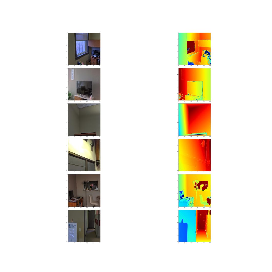
Now let’s visualize a few of our knowledge.
import matplotlib.pyplot as plt
def visualize_data(picture, depth_map, masks):
    """
    Visualizes the picture and its corresponding depth map with masks utilized.
    """
    # Apply masks to depth map
    masked_depth = depth_map * masks
    fig, axes = plt.subplots(1, 3, figsize=(15, 5))
    axes[0].imshow(picture)
    axes[0].set_title('Picture')

    # Use plt.cm.jet colormap
    axes[1].imshow(depth_map, cmap=plt.cm.jet)
    axes[1].set_title('Uncooked Depth Map')

    # Use plt.cm.jet colormap
    axes[2].imshow(masked_depth, cmap=plt.cm.jet)
    axes[2].set_title('Masked Depth Map')
    plt.savefig("visualization_example.jpg")
    plt.present()
# Instance utilization
for i in vary(3):
    img, depth_map = load_and_preprocess_data(df.iloc[i])
    # Load the masks
    mask_path = df.iloc[i]['mask']
    masks = np.load(mask_path)
    masks = cv2.resize(masks, (img.form[1], img.form[0]))  # Resize masks to match picture
    masks = np.expand_dims(masks, axis=-1)  # Add channel dimension
    visualize_data(img, depth_map, masks)
Constructing the Mannequin and Defining the Loss
Now we now have reached what may be the trickiest a part of this tutorial, however it’s attention-grabbing so sustain. For this tutorial, we are going to use an structure for the mannequin as follows.
- ResNet50 Encoder as a Spine
- 5 Decoder Layers
- An Output layer
A potential enchancment may be so as to add a bottleneck layer and optimize the decoder/encoder layers. This structure is easy and permits us to attain first rate outcomes. Let’s get to the code.
def create_depth_estimation_model(input_shape=(256, 256, 3)):
    """
    Creates a depth estimation mannequin with ResNet50 encoder and U-Internet decoder.
    """
    # Encoder
    inputs = Enter(form=input_shape)
    base_model = ResNet50(weights="imagenet", include_top=False, input_tensor=inputs)
    # Get function maps from encoder
    skip_connections = [
        base_model.get_layer("conv1_relu").output,        # (None, 128, 128, 64)
        base_model.get_layer("conv2_block3_out").output,  # (None, 64, 64, 256)
        base_model.get_layer("conv3_block4_out").output,  # (None, 32, 32, 512)
        base_model.get_layer("conv4_block6_out").output,  # (None, 16, 16, 1024)
    ]
    # Decoder
    up1 = UpSampling2D(measurement=(2, 2))(base_model.output)   # (None, 32, 32, 2048)
    concat1 = concatenate([up1, skip_connections[3]], axis=-1)  # (None, 32, 32, 3072)
    conv1 = Conv2D(1024, 3, activation='relu', padding='identical')(concat1)
    conv1 = Conv2D(1024, 3, activation='relu', padding='identical')(conv1)
    up2 = UpSampling2D(measurement=(2, 2))(conv1)   # (None, 64, 64, 1024)
    concat2 = concatenate([up2, skip_connections[2]], axis=-1)  # (None, 64, 64, 1536)
    conv2 = Conv2D(512, 3, activation='relu', padding='identical')(concat2)
    conv2 = Conv2D(512, 3, activation='relu', padding='identical')(conv2)
    up3 = UpSampling2D(measurement=(2, 2))(conv2)   # (None, 128, 128, 512)
    concat3 = concatenate([up3, skip_connections[1]], axis=-1)  # (None, 128, 128, 768)
    conv3 = Conv2D(256, 3, activation='relu', padding='identical')(concat3)
    conv3 = Conv2D(256, 3, activation='relu', padding='identical')(conv3)
    up4 = UpSampling2D(measurement=(2, 2))(conv3)   # (None, 256, 256, 256)
    concat4 = concatenate([up4, skip_connections[0]], axis=-1)  # (None, 256, 256, 320)
    conv4 = Conv2D(128, 3, activation='relu', padding='identical')(concat4)
    conv4 = Conv2D(128, 3, activation='relu', padding='identical')(conv4)
    up5 = UpSampling2D(measurement=(2, 2))(conv4)   # (None, 512, 512, 128)
    conv5 = Conv2D(64, 3, activation='relu', padding='identical')(up5)
    conv5 = Conv2D(64, 3, activation='relu', padding='identical')(conv5)
    # Output layer
    output = Conv2D(1, 1, activation='linear')(conv5)  # or 'sigmoid'
    mannequin = Mannequin(inputs=inputs, outputs=output)
    return mannequin
Using Keras and Tensorflow, we now have constructed the structure that we encompassed inside a perform. The picture measurement used right here is 256×256 so that may be elevated if wanted however it could improve the coaching time. Subsequent, we must always outline a loss perform that may optimize the mannequin because it’s coaching, for the loss perform we will go as complicated or so simple as wanted. On this tutorial, we are going to use a average method. A easy imply squared error loss perform mixed with Huber loss.
from tensorflow.keras import backend as Okay
def custom_loss(y_true, y_pred):
    mse_loss = Okay.imply(Okay.sq.(y_true - y_pred))
    huber_loss = tf.keras.losses.huber(y_true, y_pred)

    # Mix the losses
    total_loss = mse_loss + 0.1 * huber_loss
    return total_loss
Every of these losses has a weight, which we outlined to be 0.1 right here. Lastly, we have to break up the info and run it by way of our knowledge perform to feed it to the mannequin subsequent.
photographs = []
depth_maps = []
for index, row in df.iterrows():
    img, depth_map = load_and_preprocess_data(row)
    photographs.append(img)
    depth_maps.append(depth_map)
photographs = np.array(photographs)
depth_maps = np.array(depth_maps)
X_train, X_val, y_train, y_val = train_test_split(
    photographs, depth_maps, test_size=0.2, random_state=42
)
Mannequin Coaching and Inferencing
To coach the mannequin we constructed, we must compile it and match it to the info we now have.
with tf.gadget('/GPU:0'):  # Use the primary out there GPU
    mannequin = create_depth_estimation_model()
    mannequin.compile(optimizer="adam", loss=custom_loss, metrics=['mae'])
    historical past = mannequin.match(
        X_train,
        y_train,
        epochs=60,
        batch_size=32,
        validation_data=(X_val, y_val),
        shuffle=True
    )
So, right here we compile the mannequin and create it on the GPU, after which we match it. I didn’t implement many hyperparameters on this case, I used the variety of epochs to coach the mannequin, and I enabled the shuffle to try to forestall overfitting. The batch measurement is 32 which is an effective worth for our Kaggle atmosphere. There could possibly be extra hyperparameters in there, like the training price. This coaching would take round 10-Quarter-hour. Subsequent, we will outline a small perform to arrange an enter picture to check the educated mannequin.
def load_and_preprocess_image(image_path, img_size=(256, 256)):
    """Masses and preprocesses a single picture."""
    img = cv2.imread(image_path)
    img = cv2.cvtColor(img, cv2.COLOR_BGR2RGB)
    img = cv2.resize(img, img_size)
    img = tf.picture.convert_image_dtype(img, tf.float32)
    return img
new_image = load_and_preprocess_image("/kaggle/enter/keras-depth-bee-image/bee.jpg")
This can be a easy perform that does an analogous factor to what the “load_and_preprocess_data” perform did. Then we will infer the mannequin utilizing the easy line beneath.
predicted_depth = mannequin.predict(np.expand_dims(new_image, axis=0))
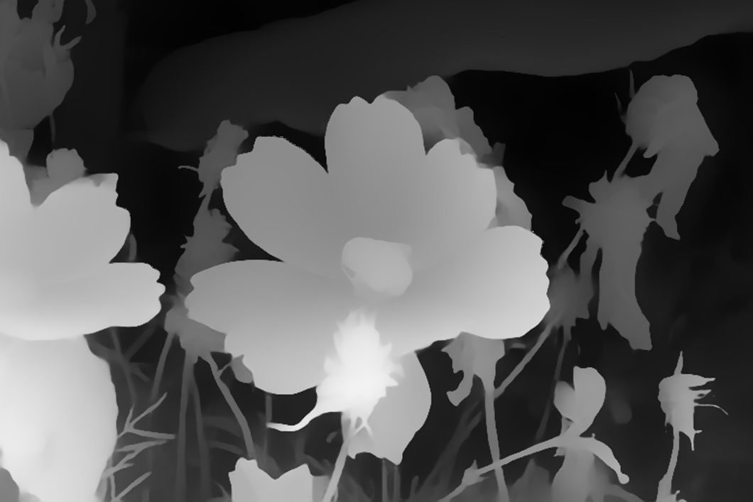
Now, we examined our picture with the educated mannequin. Let’s view the outcomes.
import matplotlib.pyplot as plt
plt.determine(figsize=(10, 5))
plt.subplot(1, 2, 1)
plt.imshow(new_image)
plt.title("Unique Picture")
plt.subplot(1, 2, 2)
plt.imshow(predicted_depth[0, :, :, 0], cmap=plt.cm.jet)  # Take away batch dimension and channel
plt.title("Predicted Depth Map")
plt.present()
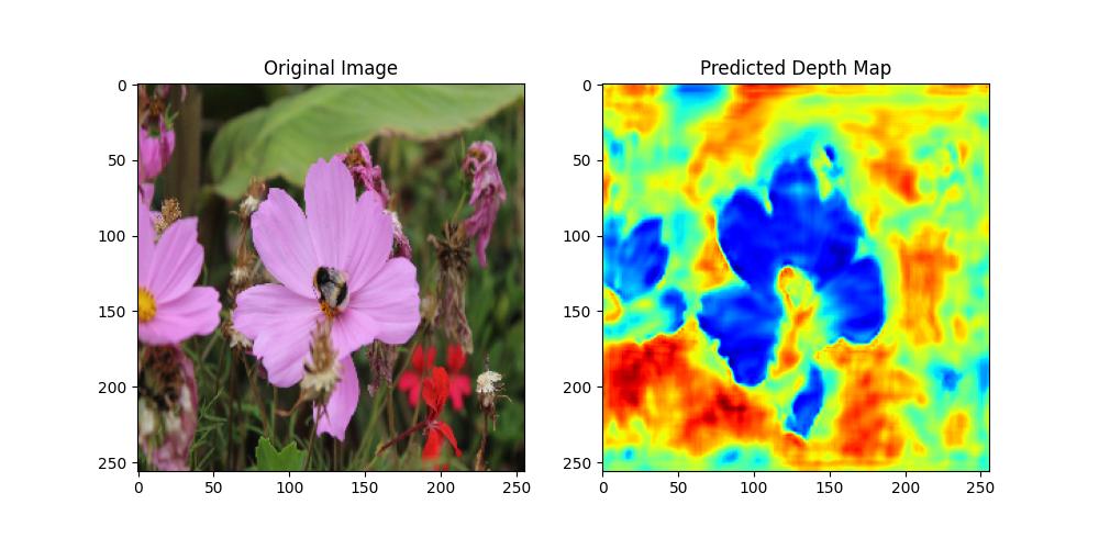
In abstract, constructing a monocular depth estimation mannequin from scratch may be an intensive process. Nevertheless, it’s a good way to study a vital process in pc imaginative and prescient. The mannequin on this tutorial is only a easy demonstration, the outcomes will not be going to be nice due to the simplicity and the shortcuts we took. Moreover, we will strive a pre-trained mannequin with just a few strains of code and see the distinction.
Inferring a Pre-Skilled Mannequin
On this part, we are going to use a easy inference on the Depth AnythingV2 mannequin, which achieves state-of-the-art outcomes on benchmark datasets like KITTI. Furthermore, to make use of this mannequin we solely want the few strains of code beneath.
from transformers import pipeline
from PIL import Picture
# load pipe
pipe = pipeline(process="depth-estimation", mannequin="depth-anything/Depth-Something-V2-Small-hf")
# load picture
url="/kaggle/enter/keras-depth-bee-image/bee.jpg"
picture = Picture.open(url)
# inference
depth = pipe(picture)["depth"]
If we save the “depth” variable we will see the results of the depth estimation which can be fairly quick contemplating that we’re utilizing the small variation of the mannequin.
With this, we now have concluded the tutorial, nonetheless, that is solely a beginning step to constructing monocular depth estimation fashions. These fashions are a large analysis space in CV and are seeing fixed enhancements. It’s because they’ve a variety of use instances, monocular depth estimation is necessary for autonomous automobiles, robotics, well being, and even agriculture and historical past.
The Future Of Monocular Depth Estimation
As we now have seen, monocular depth estimation is a difficult however necessary process in pc imaginative and prescient. Functions span from autonomous driving, robotics, and augmented actuality, to 3D modeling. The sphere remains to be enhancing, with researchers exploring new implementations and theories and pushing the boundaries. Deep studying with transformers is one promising space. This contains exploring architectures like Imaginative and prescient Transformers (ViT) which have proven promising ends in many pc imaginative and prescient duties together with monocular depth estimation.
Moreover, researchers strive integrating monocular depth estimation with different pc imaginative and prescient duties. Object detection, semantic segmentation, and scene understanding mixed with depth estimation, can create extra complete AI techniques that may work together with the world extra successfully.
The way forward for monocular depth estimation is shiny, with ongoing analysis promising to ship extra correct, environment friendly, and versatile options. As these developments proceed, we will count on to see much more revolutionary purposes emerge, remodeling industries and enhancing our interplay with the world round us.
FAQs
Q1. What’s monocular depth estimation?
Monocular depth estimation is a pc imaginative and prescient approach for estimating depth info from a single picture.
Q2. Why is monocular depth estimation necessary?
Monocular depth estimation is essential for varied purposes the place understanding 3D scene geometry from a single picture is important. This contains:
- Autonomous driving.
- Robotics.
- Augmented actuality (AR).
Q3. What are the challenges in monocular depth estimation?
Estimating depth from a single picture is inherently ambiguous, as a number of 3D scenes can produce the identical 2D projection. This makes monocular depth estimation difficult. Key challenges embrace occlusions, textureless areas, and scale ambiguity.