
Characteristic Extraction is the method of reworking uncooked knowledge, usually unorganized, into significant options, that are used to coach machine studying fashions. In right now’s digital world, machine studying algorithms are used extensively for credit score danger prediction, inventory market forecasting, early illness detection, and so on. The accuracy and efficiency of those fashions depend on the standard of the enter options. On this weblog, we are going to introduce you to characteristic engineering, why we want it and the completely different machine studying strategies out there to execute it.
What’s Characteristic Extraction in Machine Studying?
We offer coaching knowledge to machine studying fashions to assist the algorithm study underlying patterns to foretell the goal/output. The enter coaching knowledge is known as ‘options’, vectors representing the info’s traits. For instance, let’s say the target is to construct a mannequin to foretell the sale of all air conditioners on an e-commerce website. What knowledge shall be helpful on this case? It might assist to know the product options like its power-saving mode, ranking, guarantee interval, set up service, seasons within the area, and so on. Among the many sea of data out there, choosing solely the numerous and important options for enter is known as characteristic extraction.
The kind of options and extraction strategies additionally range relying on the enter knowledge sort. Whereas working with tabular knowledge, now we have each numerical (e.g. Age, No of merchandise, and categorical options (Gender, Nation, and so on). In deep studying fashions that use picture knowledge, options embody detected edges, pixel knowledge, publicity, and so on. In NLP fashions primarily based on textual content datasets, options may be the frequency of particular phrases, sentence similarity, and so on.
What’s the distinction between characteristic choice and have extraction?
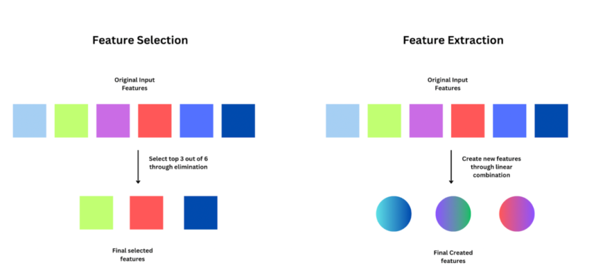
Inexperienced persons usually get confused between characteristic choice and have extraction. Characteristic choice is solely selecting the very best ‘Ok’ options from out there ‘n’ variables, and eliminating the remaining. Whereas, characteristic extraction includes creating new options by means of mixtures of the present options.

Earlier than we dive into the varied strategies for characteristic extraction, it’s essential to perceive why we want it, and the advantages it could possibly carry.
Why do we want Characteristic Extraction?
In any knowledge science pipeline, characteristic extraction is finished after knowledge assortment and cleansing. One of many easiest however correct guidelines in machine studying: Rubbish IN = Rubbish OUT! Let’s check out why characteristic engineering is required, and the way it advantages constructing a extra environment friendly and correct mannequin.
- Keep away from Noise & Redundant Info: Uncooked knowledge can have loads of noise as a consequence of gaps, and handbook errors in knowledge assortment. You may additionally have a number of variables that present the identical info, changing into redundant. For instance, if each top and weight are included as options, together with their product (BMI) will make one of many unique options redundant. Redundant variables don’t add further worth to the mannequin, as an alternative could trigger overfitting. Characteristic extraction helps in eradicating noise, and redundancy to create a strong mannequin with extracted options.
- Dimensionality Discount: Dimensionality refers back to the variety of enter options in your machine-learning mannequin. Excessive dimensionality could result in overfitting and elevated computation prices. Characteristic extraction supplies us with strategies to rework the info right into a lower-dimensional house whereas retaining the important info by lowering the variety of options.
- Improved & Quicker Mannequin Efficiency: Characteristic extraction strategies aid you create related and informative options, that present variability to the mannequin. By optimizing the characteristic set, we will pace up mannequin coaching and prediction processes. That is particularly useful when the mannequin is working in real-time and desires scalability to deal with fluctuating knowledge volumes.
- Higher Mannequin Explainability: Simplifying the characteristic house and specializing in related patterns enhance the general explainability (or interpretability) of the mannequin. Interpretability is essential to know which components influenced the mannequin’s determination, to make sure there isn’t a bias. Improved explainability makes it simpler to justify compliance and knowledge privateness rules in monetary and healthcare fashions.
With a diminished set of options, knowledge visualization strategies are more practical in capturing tendencies between options and output. Other than these, characteristic extraction permits domain-specific information and insights to be included into the modeling course of. Whereas creating options, you must also take the assistance of area specialists.
Principal Element Evaluation (PCA) for Characteristic Extraction
PCA or Principal Element Evaluation is among the extensively used strategies to battle the “curse of dimensionality”. Let’s say now we have 200 options in a dataset, will all of them have the identical influence on the mannequin prediction? No. Totally different subsets of options have completely different variances within the mannequin output. PCA goals to scale back the dimension whereas additionally sustaining mannequin efficiency, by retaining options that present most variance.
How does PCA work?
Step one in PCA is to standardize the info. Subsequent, it computes a covariance matrix that reveals how every variable interacts with different variables within the dataset. From the covariance matrix,
PCA selects the instructions of most variance, additionally known as “principal parts” by means of Eigenvalue decomposition. These parts are used to rework the high-dimensional knowledge right into a lower-dimensional house.
Implement PCA utilizing scikit study?
I’ll be utilizing a climate dataset to foretell the likelihood of rain for example to indicate the best way to implement PCA. You’ll be able to obtain the dataset from Kaggle. This dataset incorporates about 10 years of day by day climate observations from many places throughout Australia. Rain Tomorrow is the goal variable to foretell.
Step 1: Begin by importing the important packages as a part of the preprocessing steps.
# Import vital packages
import numpy as np
import pandas as pd
import seaborn as sb
import matplotlib.pyplot as plt
from sklearn import preprocessing # To get MinMax Scaler perform
Step 2: Subsequent, learn the CSV file into an information body and cut up it into Options and Goal. We’re utilizing the Min Max scaler perform from sklearn to standardize the info uniformly.
# Learn the CSV file
knowledge = pd.read_csv('../enter/weatherAUS.csv')
# Break up the goal var (Y) and the options (X)
Y = knowledge.RainTomorrow
X = knowledge.drop(['RainTomorrow'], axis=1)
# Scaling the dataset
min_max_scaler = preprocessing.MinMaxScaler()
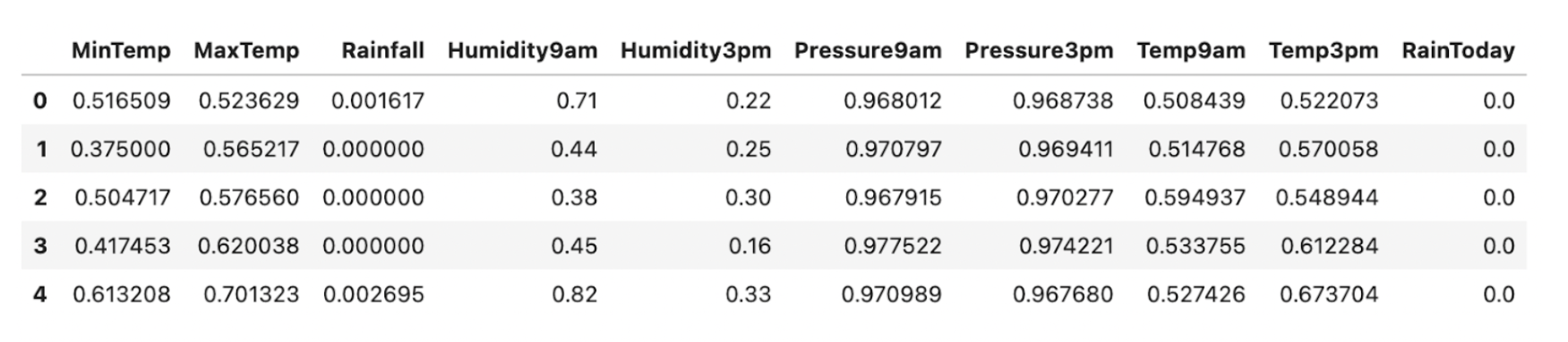
X_scaled = pd.DataFrame(min_max_scaler.fit_transform(X), columns = X.columns)
X_scaled.head()
Step 3: Initialize the PCA class from sklearn.decomposition module. You’ll be able to cross the scaled options to ‘pca.match()’ perform as proven beneath.
# Initializing PCA and becoming
from sklearn.decomposition import PCA
pca = PCA()
pca.match(X_scaled)
PCA will then compute the variance for various principal parts. The ‘pca.explained_variance_ratio_’ captures this info. Let’s plot this to visualise how variance differs throughout characteristic house.
plt.plot(pca.explained_variance_ratio_, linewidth=2)
plt.axis('tight')
plt.xlabel('Variety of Feautres')
plt.ylabel('Variance Ratio')
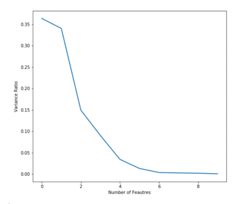
From the plot, you’ll be able to see that the highest 3-4 options can seize most variance. The curve is nearly flat past 5 options. You’ll be able to this plot to determine what number of closing options you wish to extract from PCA. I’m selecting 3 on this case.
Step 4: Now, initialize PCA once more by offering the parameter ‘n_components’ as 3. This parameter denotes the variety of principal parts or dimensions that you just’d like to scale back the characteristic house to.
pca = PCA(n_components=3)
pca.fit_transform(x_train)
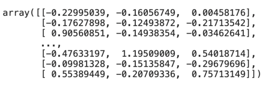
We now have diminished our dataset to three options as proven above. If you wish to test the whole variance captured by the chosen parts, you’ll be able to calculate the sum of the defined variance.
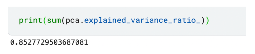
The diminished set of three options captures 85% variance amongst all options!
It’s finest to make use of PCA when the variety of options is just too large to visualise or interpret clearly. PCA may deal with multilaterally, however it’s delicate to outliers current. Guarantee the info is cleaned by eradicating outliers, scaling, and standardizing.
LDA for Characteristic Extraction
Linear Discriminant Evaluation (LDA) is a statistical approach extensively used for dimensionality discount in classification issues. The goal is to discover a set of linear mixtures of options that finest separate the courses within the knowledge.
How is LDA completely different from PCA?
PCA targets solely maximizing knowledge variance, which is finest in regression issues. LDA targets to maximise the variations between courses, which is right for multi-classification issues.
Let’s take a fast look into how LDA works:
- LDA requires the enter knowledge to be usually distributed and computes covariance matrices
- Subsequent, LDA calculates two varieties of scatter matrices:
- Between-class scatter matrix: It’s computed to measure the unfold between completely different courses.
- Inside-class scatter matrix: It computes the unfold inside every class.
- Eigenvalue Decomposition: LDA then performs eigenvalue decomposition on the matrix to acquire its eigenvectors and eigenvalues.
- The eigenvectors similar to the most important eigenvalues are chosen. These eigenvectors are the instructions within the characteristic house that maximize class separability. We challenge the unique knowledge throughout these instructions to acquire the diminished characteristic house.
Implement LDA on Classification Duties?
Let’s create some artificial knowledge to play with. You should use the ‘make_classification()’ perform from scikit study for this. Discuss with the code snippet beneath. As soon as the info is created, let’s visualize it utilizing a 3D plot.
from sklearn.datasets import make_classification
options, output = make_classification(
   n_features=10,
   n_classes=4,
   n_samples=1500,
   n_informative=2,
   random_state=5,
   n_clusters_per_class=1,
)
# Plot the 3D visualization
fig = px.scatter_3d(x=X[:, 0], y=X[:, 1], z=X[:, 2], colour=y, opacity=0.8)
fig.present()
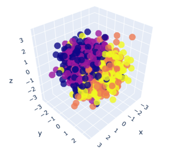
Within the visualization, we will see 4 completely different colours for every class. It appears unattainable to search out any patterns at present. Subsequent, import the LDA module from discriminant_analysis of scikit study. Much like PCA, it’s essential to present what number of diminished options you need by means of the ‘n_components’ parameter.
From sklearn.discriminant_analysis import LinearDiscriminantAnalysis
# Initialize LDA
lda = LinearDiscriminantAnalysis(n_components=3)
post_lda_features = lda.match(options, output).remodel(options)
print("variety of options(unique):", X.form[1])
print("variety of options that was diminished:", post_flda_features.form[1])
OUTPUT:
>> variety of options(unique): 10
>> variety of options that was diminished: 3
We now have efficiently diminished the characteristic house to three. You can even test the variance captured by every characteristic utilizing the beneath command:
lda.explained_variance_ratio_

Now, let’s visualization the diminished characteristic house utilizing the beneath script:
fig = px.scatter(x=post_lda_features[:, 0], y=post_lda_features[:, 1], colour=y)
fig.update_layout(
   title="After LDA on characteristic house",
)
fig.present()
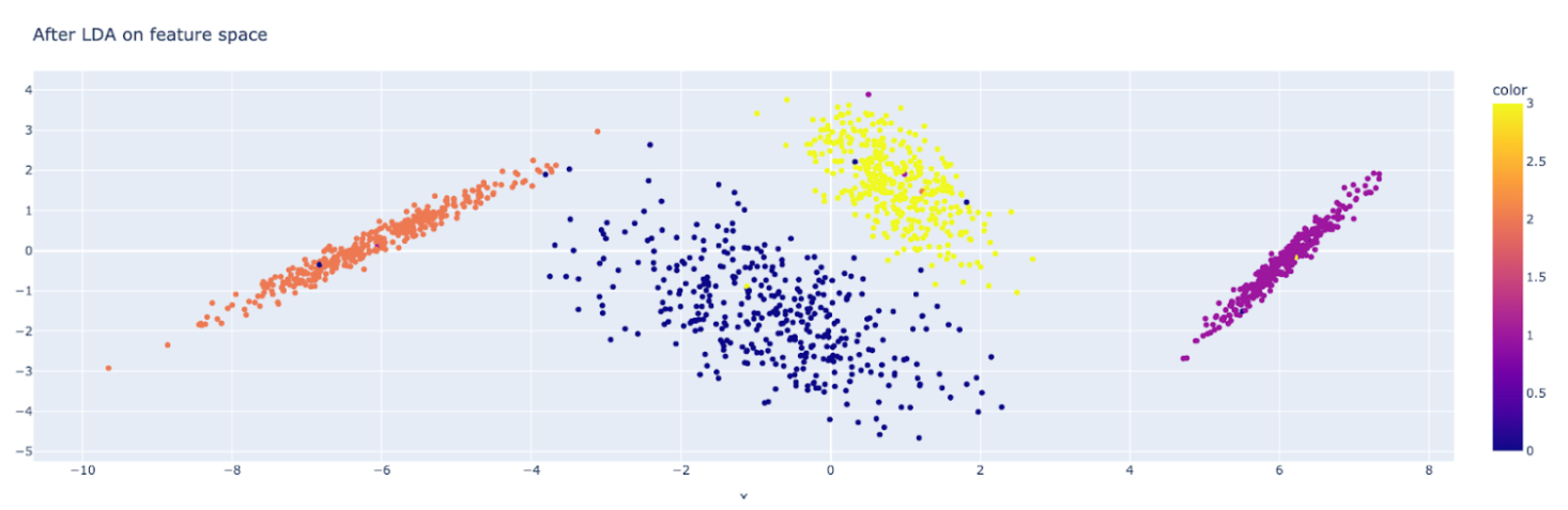
You’ll be able to clearly see how LDA helped in separating the courses! Be at liberty to experiment with a distinct variety of options, parts, and so on.
Characteristic Extraction with t-SNE
t-SNE stands for t-distributed Stochastic Neighbor Embedding. It’s a non-linear approach and is most popular for visualizing high-dimensional knowledge. This technique goals to protect the connection between knowledge factors whereas lowering the characteristic house.
How does the algorithm work?
First, every knowledge level within the dataset is represented by a characteristic vector. Subsequent, t-SNE calculates 2 likelihood distributions for every pair of knowledge factors:
- The primary distribution represents the similarities between knowledge factors within the high-dimensional house
- The second distribution represents the similarities within the low-dimensional house
The algorithm then Minimizes the distinction between the 2 distributions, utilizing a value perform. Mapping to decrease dimensions: Lastly, it maps the info factors to the lower-dimensional house whereas preserving the native relationships.
Right here’s a code snippet to rapidly implement t-SNE utilizing scikit study.
from sklearn.manifold import TSNE
tsne = TSNE(n_components=3, random_state=42)
X_tsne = tsne.fit_transform(X)
tsne.kl_divergence_
Let’s rapidly plot the characteristic house diminished by t-SNE.
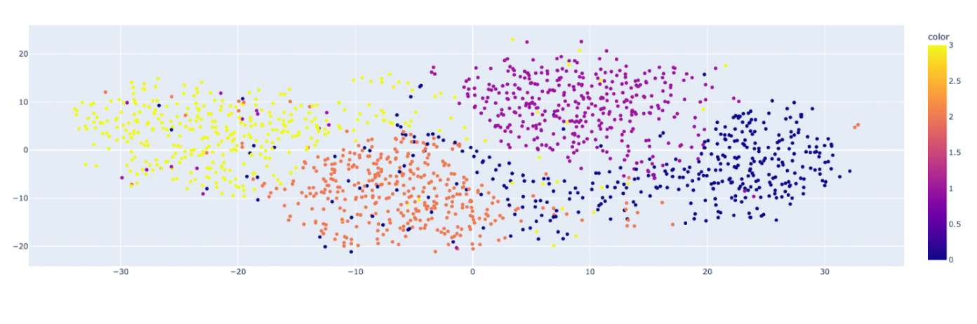
You’ll be able to see the clusters for various courses of the unique knowledge set and their distribution. Because it preserves native relationships, it’s the finest technique for visualizing clusters and patterns.
Specialised Characteristic Extraction Methods
The strategies mentioned above are for tabular knowledge. Whereas coping with textual content or picture knowledge, now we have specialised characteristic extraction strategies. I’ll briefly go over some standard strategies:
- Characteristic Extraction in Pure Language Processing (NLP): NLP fashions are constructed on massive corpora of textual content knowledge. Bag-of-Phrases (BoW) is a way that Represents textual content knowledge by counting the frequency of every phrase in a doc. Time period Frequency-Inverse Doc Frequency (TF-IDF) can be used. Methods like Latent Dirichlet Allocation (LDA) or Non-Destructive Matrix Factorization (NMF) are helpful for extracting matters. They’re utilized in NLP duties like doc clustering, summarization, and content material suggestion.
- Characteristic Extraction in Pc Imaginative and prescient: In laptop imaginative and prescient, duties like picture processing classification, and object detection are very talked-about. The Histogram of Oriented Gradients (HOG) Computes histograms of gradient orientation in localized parts of a picture. Characteristic Pyramid Networks (FPN) can mix options at completely different resolutions. Scale-Invariant Characteristic Remodel (SIFT) can detect native options in photographs, sturdy to modifications in scale, rotation, and illumination.
Conclusion
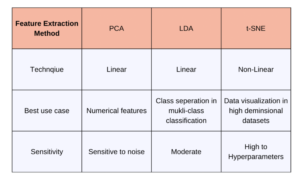
Characteristic extraction is a vital a part of getting ready high quality enter knowledge and optimizing the sources. We will additionally reuse pre-trained characteristic extractors or representations in associated duties, saving large bills. I hope you had a very good learn on the completely different strategies out there in Python. When deciding which technique to make use of, take into account the particular targets of your evaluation and the character of your knowledge. If you’re primarily enthusiastic about lowering dimensionality whereas retaining as a lot variance as potential, PCA is an efficient selection. In case your goal is to maximise class separability for classification duties, LDA could also be extra acceptable. For visualizing advanced numerical datasets and uncovering native buildings, t-SNE is the go-to selection.