Introduction to Uncertainty in Machine Learning Models: Aleatoric Uncertainty with TensorFlow Probability

Aleatoric uncertainty is a key a part of machine studying fashions. It comes from the inherent randomness or noise within the information. We will not scale back it by getting extra information or tweaking the mannequin design. Visualizing aleatoric uncertainty helps us perceive how the mannequin performs and the place it is uncertain. On this submit, we’ll discover how TensorFlow Likelihood (TFP) can visualize aleatoric uncertainty in ML fashions. We are going to give an summary of aleatoric uncertainty ideas. We’ll embody clear code examples and visuals displaying how TFP captures and represents aleatoric uncertainty. Lastly, we’ll talk about the true advantages of visualizing aleatoric uncertainty in ML fashions. we’ll additionally spotlight circumstances the place it will possibly assist decision-making and enhance efficiency.

Visualizing Aleatoric Uncertainty utilizing TensorFlow Likelihood

TensorFlow Likelihood (TFP) enables you to carry out probabilistic modeling and inference utilizing TensorFlow. It is received instruments for constructing fashions with likelihood distributions and probabilistic layers. With TFP, you may see the uncertainties in your machine studying fashions, which is tremendous useful.

Let’s take a look at an instance – the MNIST dataset with handwritten digits. We’ll use a convolutional neural web (CNN) to categorise the pictures, after which, we are able to mannequin the CNNs output as a categorical distribution with TFP. Here is some code to point out the way it works:

import tensorflow as tf
import tensorflow_probability as tfp
import matplotlib.pyplot as plt

# Outline the mannequin
mannequin = tf.keras.Sequential([
    tf.keras.layers.Conv2D(32, (3, 3), activation='relu', input_shape=(28, 28, 1)),
    tf.keras.layers.MaxPooling2D((2, 2)),
    tf.keras.layers.Flatten(),
    tf.keras.layers.Dense(10),
])

# Load the MNIST take a look at set
test_images, test_labels = tf.keras.datasets.mnist.load_data()[1]

# Preprocess the take a look at set
test_images = test_images.astype('float32') / 255.
test_images = test_images[..., tf.newaxis]

# Make predictions on the take a look at set
predictions = mannequin.predict(test_images)

# Convert the predictions to a floating-point sort
predictions = predictions.astype('float32')

# Convert the predictions to a TensorFlow Likelihood distribution
probs = tfp.distributions.Categorical(logits=predictions).probs_parameter().numpy()

# Get the anticipated class labels
labels = tf.argmax(probs, axis=-1).numpy()

# Get the aleatoric uncertainty
uncertainty = tf.reduce_max(probs, axis=-1).numpy()

# Visualize the aleatoric uncertainty
plt.scatter(test_labels, uncertainty)
plt.xlabel('True Label')
plt.ylabel('Aleatoric Uncertainty')
plt.present()

• Import the required libraries: We had to herald the correct libraries – TensorFlow and TensorFlow Likelihood for working with likelihood and inference, and Matplotlib to show the information visually.
• Outline the mannequin: A Sequential mannequin is outlined utilizing Keras, which is a plain stack of layers the place every layer has precisely one enter tensor and one output tensor. The mannequin consists of a convolutional layer with 32 filters of measurement (3,3), a max pooling layer, a flatten layer, and a dense layer with 10 models.
• Load the MNIST take a look at set: We used Keras to load up the MNIST take a look at photographs of handwritten numbersI used Keras to load up the MNIST take a look at photographs of handwritten numbers
• Preprocess the take a look at set: We preprocessed by normalizing the pixel values between 0 and 1 and including a brand new axis to make them suitable with the mannequin.
• Make predictions on the take a look at set: We ran the take a look at photographs by means of the mannequin to get predictions.
• Convert the predictions to a floating-point sort: The predictions are transformed to a floating-point sort to make them suitable with the TFP distribution.
• Convert the predictions to a TensorFlow Likelihood distribution: Utilizing TFP’s Categorical, we turned the predictions into likelihood distributions over the courses.
• Get the anticipated class labels: We get the anticipated class labels by taking the category with the best predicted likelihood for every information level.
• Get the aleatoric uncertainty: To measure the inherent randomness within the mannequin’s predictions, we take a look at the utmost predicted likelihood for every information level. That is known as the aleatoric uncertainty.
• Visualize the aleatoric uncertainty utilizing a scatter plot: To visualise the uncertainty, we are able to make a scatter plot with the true labels on x-axis and the aleatoric uncertainty values on the y-axis. This allows you to see how the uncertainty varies throughout completely different information factors and completely different true courses. Factors with low most possibilities could have excessive aleatoric uncertainty and seem greater on the plot.

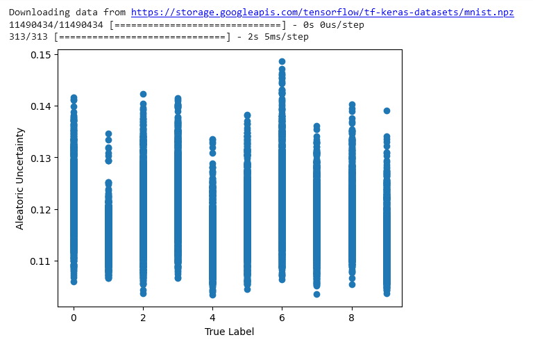
The plot from the code reveals how the true label pertains to the aleatoric uncertainty. The x-axis represents the true digit within the picture – the true label. And the y-axis represents the utmost likelihood from the anticipated distribution – that is the aleatoric uncertainty.

The aleatoric uncertainty captures the randomness or noise within the information utilizing a likelihood distribution for the mannequin’s predictions. Excessive uncertainty means the mannequin’s not very assured in its prediction. Low uncertainty signifies that the mannequin is fairly certain of the prediction.

Trying on the plot might help to know how effectively the mannequin is working and the place it struggles. For instance, excessive uncertainty for some true labels may point out that the mannequin is struggling to make correct predictions for that vary of labels.

Conclusion

TensorFlow Likelihood (TFP) is a reasonably useful library that permits you to visualize the inherent randomness (additionally known as aleatoric uncertainty) in machine studying fashions. With TFP, you may construct fashions that really output likelihood distributions. That is helpful as a result of it provides you a way of how uncertain the mannequin is about its predictions. In the event you visualize these likelihood distributions in a scatter plot, you may actually see the uncertainties. Wider distributions imply extra uncertainty – the mannequin is not very assured. Tighter distributions imply decrease uncertainty – the mannequin is fairly certain of the prediction.

Visualizing aleatoric uncertainty might help us perceive how effectively the mannequin is working and the place it struggles. As an illustration, you may see excessive uncertainty for some true labels telling you the mannequin is having hassle in that space of the enter area. Or possibly the uncertainty is low throughout the board apart from a couple of stray information factors – may these be mislabeled within the coaching information? The purpose is, visualizing aleatoric uncertainty opens up potentialities for debugging and bettering your fashions.